Sunday, January 14, 2018

Chess Analytics: Cluster analysis & Patterns of time usage in 10-min games

In this installment of Chess Analytics, I've decided to investigate the question: What are the distinct patterns of time usage during 10-minute online chess games? In doing so, we will also attempt to determine just how many distinct patterns we can distinguish.


Cluster Analysis

To attempt to answer this question, we can use cluster analysis. Cluster analysis is possibly also known as "segmentation analysis" or "taxonomy analysis", though I am not familiar with those terms.

Through cluster analysis, we can group chess games into similar (homogeneous) subgroups, based on how similar the games are on certain variables. The goal of cluster analysis is to obtain games that are very similar within groups, and very different between groups (if that's at all possible). So to examine patterns of time usage during online chess games, we can calculate the time taken at each move by the players, and perform a cluster analysis on those time values. This will give us subgroups of games that are similar in the time taken at each move.

If you're familiar with machine learning, you'll know that cluster analysis is a type of "unsupervised" learning algorithm: The algorithm will categorize the chess games in different groups without having known beforehand which group the games belong to (we just don't know what they are yet!). The term unsupervised is used to contrast with "supervised" learning algorithms, in which the algorithm learns to categorize observations based on a sample of observations that have already been categorized into groups.


The Data

To look at the patterns of time usage in chess games, I used the first 200 MB of the rated games played in October 2017 on the internet chess server lichess, retaining only those games for which the computer evaluation of each move was available (this was not necessary for this particular analysis, but this same dataset could be used for other analyses as well). In total, this gave us 7,387 games. However, because the current investigation is about time usage, I restricted the analysis to those games whose time control was 10 minutes in total, with or without increment (for example, 10+0, or 4+9), and which lasted at least 25 moves, so as to look at the patterns in the first 25 moves of the game. So in the end, a total of 843 games fit those criteria. The goal of this analysis is to group those 843 games into homogeneous subgroups of games that are similar in their patterns of time usage.

To give you an idea of what the dataset looks like, here's a screenshot of the first few rows (this is a Pandas DataFrame in Python):


Because of the likely relationship between the time taken at each move by both players during the game, here we focus on the time pattern for White players (but the results were similar when looking at the Black side instead). The first column, clocks_diff_31, indicates the difference in the remaining time of the White player (in seconds) between the third ply (i.e., White's second move) and the first ply (i.e., White's first move). In other words, the first column gives the number of seconds White spent on their second move. Analogously, the second column, clocks_diff_53, indicates the time taken by White between the third and fifth ply (i.e., during White's third move), and so on, up to the 25th move. Note that on lichess, the clock only starts ticking at the second move, so we don't have access to the time taken during the first move for these games.


Number of Patterns & Hierarchical Clustering

Perhaps the most important decision that goes into a cluster analysis is choosing the number of clusters to detect, or in this case, the number of distinct patterns of time usage we can distinguish in the games. One data-driven way to do this is through hierarchical clustering, where chess games are grouped two by two based on the similarity of their pattern of time usage, then these new pairs are grouped with another pair again based on similarity, and so on, until only one big cluster--containing all the games--is created. In this way, clusters are formed sequentially, and we can decide where to stop the clustering.

We can visualize this hierarchical clustering through a dendrogram (don't do like me and misspell it "dendogram" every time!). A dendrogram shows which games are being grouped together due to their similar time-usage patterns at each iteration of the process, starting with no clusters at the bottom, and one giant cluster that includes all games at the top.

Here is a simple example of a dendrogram (courtesy of StackExchange):


In this dendrogram, 10 observations (or if you prefer in our case, 10 chess games) are being sequentially grouped. The horizontal x axis indicates the game index (which is arbitrary), and the vertical y axis indicates the dissimilarity between games within a cluster (i.e., the "distance" between games). Starting from the bottom of the dendrogram, we can see that games #2 and #10 are most similar in their pattern (the distance between them is the smallest at < 0.2) and are grouped together first. Next games #5 and #8 are grouped; then games #7 and #6; then game #9 is most similar to the "average" of games #5 and #8 and so is grouped with that cluster; and so on until the cluster formed by games #3, #7, and #6 is combined with the cluster formed by the other games.

Choosing the number of clusters means choosing a maximum difference (or distance) between games within each cluster, as represented by the y axis. So in the simple example above, we could decide that 4 clusters is appropriate by drawing a horizontal line somewhere around a distance of 0.6, thereby yielding the following clusters: (1) game #3; (2) games #7 and #6; (3) games #1 and 4; and (4) games #2, 5, 8, and 10.

Evidently, the current analysis--with 843 chess games rather than 10--yields a much more dense dendrogram (click on the picture to resize):


Based on this dendrogram, a reasonable choice for the number of patterns seems to be 3, and if the three-cluster solution yields patterns that are difficult to interpret, then another reasonable choice is 2. (The Python library that generated this dendrogram seems to suggest 2 clusters, given the color coding.) The dendrogram might also lead us to conclude that 4 clusters is not very reasonable, as the distance between the third and fourth clusters would be very small.

The good news is that nothing prevents us from trying out several alternatives. A convenient way to choose the number of clusters is to try a few reasonable numbers and choose one that yields groupings that make sense given the context (here, time usage patterns) all the while providing groups with a large-enough size (a cluster that includes only a handful of games is not very useful). In some applications, obtaining clusters of approximately equal sizes is desirable, but that's not really the case here. So we can try out 3 clusters, and also examine the two-cluster solution in case it ends up being more interesting or interpretable.


Three Patterns of Time Taken During a 10-Min Game

The graph below shows the three distinct patterns of time usage detected in a three-cluster cluster analysis. The graph shows the median time taken at each move, so that 50% of the games of a given group took less time than is shown on the graph, and 50% of the games took more time than is shown. In total, 158 games were categorized in pattern #1; 438 games were categorized in pattern #2; and 247 games were categorized in pattern #3.


Let's try to describe these patterns. It looks like they are not too surprising and make sense. Pattern #3 (green line at the bottom) represents games that are played rather quickly throughout, with perhaps a slight increase in move time as the game goes on. Pattern #1 (blue line at the top), on the other hand, represents games that are played much more slowly, especially starting around move 7-8, with some peaks a little bit later in the game; these games also seem to pick up the pace again after move 15, but it's difficult to say given that our analysis ends at move 25. Finally, Pattern #2 (orange line in the middle) represents games that are in-between the faster-paced and slower-paced games of Patterns #1 and #3.

Note that the graph showing the average time taken at each move (rather than the median time) is nearly identical to this one.

The three patterns of time usage found above are easy to interpret and make sense. To make sure that we're not missing out on a better solution, let's do as promised and look at the two-pattern solution. We get the following graph, which again shows median time taken at each move in each pattern:


Pattern #2 (orange line on top) is exactly the same as Pattern #1 above (represented by the same 158 games as before). This is because this pattern is the pattern that is most different from the other patterns (see the games in green on the left of the dendrogram above). With the two-pattern solution, the two faster patterns are now combined into Pattern #1 (blue line at the bottom), with a total of 685 games (i.e., the sum of 438 + 247 games from Patterns #2 and #3 in the three-pattern solution). These two patterns are also simple and easy to interpret, but nothing is gained from the three-pattern solution; in fact, we've lost the distinction between the faster-paced games in terms of their pattern of time taken. So I prefer the three-pattern solution here.


Conclusion from the Cluster Analysis on Time Patterns in 10-Min Games

Overall, from the cluster analysis above we could draw the conclusion that there are 3 general patterns that 10-minute online chess games follow in terms of time usage:
  1. Games that are faster-paced in the opening but that slow down noticeably at the end of the opening (around move 8; this is Pattern #1 in the three-cluster cluster analysis);
  2. Games that are relatively fast throughout, though slightly longer after the opening (this is Pattern #3 in the three-cluster cluster analysis);
  3. Games that are neither fast nor slow, and whose moves also tend to slow down slightly after the initial opening moves.


What's Next?

This analysis was limited to some 800 online games played in October 2017 on lichess.org. I doubt that patterns would change much over time (say if we were to do this analysis again in October 2018), but perhaps patterns do change by chess servers (maybe players are more or less impatient on chess.com, for example?), and my guess is that patterns are different in over-the-board games rather than online games. (If you have a good dataset for OTB games, please let me know.) This analysis also doesn't show what happens beyond the 25th move, for example during endgames.

Another unanswered question that seems interesting is the relationship between pattern of time taken and game outcome. However, not only might the effect of time usage on game outcome vary from player to player, but there probably is a very strong relationship between time taken at each move by White and time taken by Black. Nonetheless, one (odd) possibility is that some patterns are associated with more wins for White, while other patterns are associated with more wins for Black... I haven't checked, but I do think it would be very odd!

Friday, January 5, 2018

Transposition Gone Wrong: Attempting to reach the Benko Gambit

Happy New Year! May 2018 bring us the best chess... Also, fame and fortune.

I love playing the Benko Gambit as Black, so I try to reach it whenever I can. But it doesn't always go so smoothly. Normally the Benko Gambit is reached after 1. d4 Nf6 2. c4 c5 3. d5 b5:


Typically White will play cxb5 at some point, and Black will respond with a6 (a pawn gambit), and White can choose to take the pawn with bxa6 (gambit accepted--the most common response) or to push with b6 (gambit declined). When the gambit is accepted, Black will fianchetto the king's bishop, put the knight on f6, play d6 (some players prefer e6), castle kingside; White will typically get e2-e4 in (even though this is not an e4 opening). A position like this might arise:


Black will eventually recapture the a6 pawn, and White will have a passed a-pawn, but Black will have tremendous activity on the queenside, with moves like Bxa6, Nbd7, Qb6, Rfb8 (after Black castles kingside), etc. Note that in the "old main line", which I don't particularly fancy, Black plays Bxa6 before White plays e4, so that when White plays e4, Black responds with Bxf1, and White plays Kxf1 and will manually castle their king with g3 and Kg2.

I've had quite a bit of success playing the Benko as Black. This graph shows the win percentage (in green), draw percentage (in blue), and loss percentage (in red) by opening when I play a rapid or classical game (> 8 minutes) as Black on lichess.org. In fact, my highest win percentage comes from games where I've played the Benko (10 games, win percentage = 80%; see middle of the graph):


So I'm somewhat justified in trying to reach this opening when I can. Against 1. e4, there are a few ways to try to reach this opening. An uncommon one is the St. George defense, with 1. e4 a6 (since both e4 for White and a6 for Black are moves in Benko lines). A more common opening that allows one to hope to reach a Benko position is the Robtasch (or "Modern") defense with 1. e4 g6, which is what I played in this game (incidentally, notice that the Robatsch seems to be one of my worst openings in the graph above). In this game I was facing a stronger opponent (2142 blitz on chess.com), and we reached the following position after 1. e4 g6 2. d4 Bg7 3. Nf3 a6 4. c4 d6 5. Nc3 Nd7 6. Be2 c5:


Up to here I've played all moves that are consistent with the Benko so that I can transpose into it were the opportunity arise. And we're really close to it: If White plays d5, I'll respond with b5 and we will have reached a position consistent with the Benko gambit. But my opponent doesn't have to humor me, and indeed he chose not to, and simply played 7. O-O. But I was not ready to give up though I should have been, and I played 7. ... b5? 8. cxb5:


And here I played a move that would simply be impossible to play in the Benko gambit since White would have played d5 earlier. I played the ridiculous-looking 8. ... cxd4?! 9. Nxd4 axb5?? (9. ... a5) 10. Bxb5:


And once the smoke has cleared, this is not a Benko gambit, and White has two connected passed pawns on the queenside! (With a normal Benko gambit White would only have a passed a-pawn.) Stockfish gives White a two-pawn advantage at this point, and my opponent went on to kick my butt. I later gave up one of my knights for his two pawns but it was already too late.

So, lesson learned: Don't part with all three of the c-, b-, and a-pawns in the Benko Gambit, because White will have two connected passed pawns on the queenside. It seems obvious, but I had to learn the hard way.

The full game is available here:

Friday, December 29, 2017

Problem #10

I found this puzzle on lichess.org, and failed to find the solution. White to play:


[Show solution]

Thursday, November 30, 2017

Problem #9

The position below was reached after 22. ... e4 in a 90+30 game on lichess (full game is below). Black played e5 to defend against Rd3+. A few people were spectating the game, and one user found, several minutes later, the best move that could have been played in this position. It's such an unexpected move that at first I thought the user was kidding...


[Show solution]


The full game is available here (White missed the best move at move 23):


Tuesday, November 21, 2017

My queen is invisible #3

This is the third installment of this series! Why isn't my queen taken seriously!!! I can do stuff with it.

I played a 2+0 casual game on lichess.org against a player who I had lost against previously, so I was thrilled to get a shot at revenge. I reached the position below from a Caro–Kann defense, my opponent just played 13. dxc5:


I can't immediately take back the pawn, and my opponent is threatening to play b4 to protect it, so I played 13. ... a5 14. a3 (once again threatening b4) 14. ... a5, preventing b4 once more (or so I thought). My opponent decided to play 15. b4?! anyway:


I took with 15. ... axb3 16. Qxb3, and here in an attempt to regain the pawn I played 16. ... Qa5:


It might look like the b7 pawn is hanging with Qxb7, but then I would have Qxc3+, so the pawn is poisoned. My opponent tried to hold his pawns together by playing 17. Bd4, but this does nothing to protect c4, so I took with 17. ... Bxc5, still having in mind that 18. Bxc5 Qxc5 19. Qxb7 would leave the c3 pawn hanging with check. But just when I thought the b7 pawn was poisoned, my opponent took it with 18. Qxb7?:


This is a blunder a simply loses a piece on d4, since the c3 pawn is pinned to the king by the queen. So I played 18. ... Nxd4 (18. ... Bxd4 19. Qxc6+ loses):


Stockfish recommends for white to give up the piece on d4 and castle kingside. But my opponent, as many of my opponents do, went for the double-rook sweep (or whatever), and played 19. Qxa8+?? Qxa8 0-1. Stockfish does concede that this variation wins back the piece on d4 however.

The game is available in full here:


Monday, November 13, 2017

Taking full advantage of a bad tactic

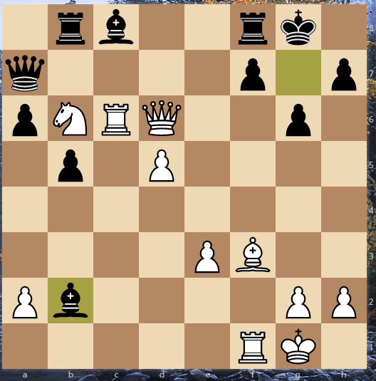
I reached the dominating position below in a casual 10 3 game on lichess after 20. Nb6 Qa7:


Here my knight on b6 is attacked, but my b2 pawn is also threatened by the bishop on g7. I could try to defend both with, for instance, 21. Nxc8 Rbxc8 22. b3, but I didn't want to give up my knight for the c8 bishop, which has very limited scope right now (it can't develop to b7 because of Rc7 or to f5 because of e4). I also didn't want to give up the control of the c-file. So instead I sacrificed the b2 pawn and played 21. Rc6 (defending the knight, and perhaps preparing Rfc1) 21. ... Bxb2:


I wasn't sure how to best play this position. Of course 22. Rfc1 is not immediately possible. I'm still trying to prevent Black from activating his pieces, and the best way to do this is to prevent Black from developing the c8 bishop, which is also preventing the rooks from being connected. So I played 22. Kh1, so that I can play e3-e4 if Black attempts Bf5 (Bb7 is still not a good idea in view of Rc7). Next I can think of playing Rf2-c2 or even e3-e4-e5. But my opponent tried a bad tactic here, he played 22. ... Ba6?:


The goal of this move was to free his position with 23. Qxa3 Rxb6, exchanging my forward knight for his dark-squared bishop. I successfully took advantage of this mistake, but it turns out there was a slightly better continuation which I had dismissed early on in my calculations. Here I played the simple 23. Nxc8 Bxd6 24. Nxa7, which won a piece (Black continued with 24. ... Ra8 25. Rxd6 Rxa7, though Stockfish recommends 24. ... Rfd8 instead).

But I had a better way to take advantage of 22. ... Ba6. I could simply play 23. Qxa3!, which I had dismissed because of the obvious 23. ... Rxb6, but here White has the move 24. Qc4!:


And Black would have been forced to play 24. ... Rb7 (safeguarding the rook), which loses the bishop after 25. Rxc8. The passed d pawn is ready to be pushed, which would also open up the attack of the f3 bishop onto the b7 rook.

For what it's worth, the difference in Stockfish evaluations between my continuation and the best continuation is about 2 pawns, ~+4.2 vs. ~+6.1.

The full game is available here:


Monday, November 6, 2017

Chess Analytics: Predicting rating from average centipawn loss

I have had the idea of trying to derive a player's rating "empirically", through their play rather than through their results (as is currently done). As a starting point, I thought that it might be possible to approximate a player's rating by looking at their average centipawn loss. The average centipawn loss (aCPL) is the amount by which a chess engine's evaluation of the position changes after each of the player's moves. For example, if the score is about +1.20 before White's move, and White plays a small mistake and the evaluation is +0.30 after White's move, then White's centipawn loss for that move is +1.20 - +0.30 = +0.90; the average centipawn loss is the mean CPL over the course of the game. I thought that perhaps stronger players would have a lower aCPL, such that it would be possible to approximate a player's rating from their aCPL.

The Data

To investigate this question, I downloaded one of the databases available on lichess.org. These databases include all rated games played on lichess for a given period. For the purposes of this exercise, I used a subset of the August 2014 database. From these games, I kept only the ones for which computer analysis was available, so that the engine's evaluation--here, Stockfish--is available after each half-move.

I used Python to transform the file of PGNs into a dataset amenable to statistical analysis. In this dataset, each row is a different game (i.e., a different PGN in the database downloaded on lichess). The figure below shows the first few columns and rows of the dataset:


As you can see, all the meta data for each PGN is kept, and the tags (like "WhiteElo", "Event", etc.) are used as column names. I had to perform operations on the "Moves" column in order to extract the evaluation at each ply. The resulting variables (up to 200 half-moves in this particular dataset) look like this:


Here, I've limited my attention to evaluations ranging from -3 to +3 to avoid getting statistics that are too influenced by extreme scores; any evaluations greater than +3 or less than -3 have been removed (however, the results presented below are very similar whether or not the full range is included, so this is more of a detail at present). From there, I've calculated the difference between each evaluation and the preceding one; half of those differences represents the centipawn loss for the white player, and the other half represents the centipawn loss for the black player. The resulting variables look like this:


Finally, for each game, it is possible to calculate the average centipawn loss for each player by averaging those difference variables across rows, yielding the two aCPL variables:


Descriptive Statistics

Now that the data are ready for analysis, I looked at some descriptive statistics for the variables of interest, the white and black ratings and aCPL. For the final dataset, the average rating for the white players was 1637 (SD = 238), and the average rating for the black players was 1630 (SD = 239). The average aCPL for the white and black players were also very similar, with 0.26 (SD = 0.16) for white and 0.24 (SD = 0.14) for black (again, this is only looking at positions in which the evaluation was between -3.00 and +3.00)

Here's a histogram showing the frequency at which each aCPL is observed in the sample (separated by colors), along with the corresponding kernel density estimation plot:


As can be seen in the second figure, the vast majority of players (with these transformed data) had a relatively low aCPL, below 0.50. This is to be expected, since players with even higher aCPLs would quickly lose almost every game.

Visually, it's also possible to inspect the relationship between aCPL and rating through a scatterplot:


The horror! Even before jumping into the modeling, our guess is that there is not a strong relationship between aCPL and rating! Observations are relatively tightly distributed on the x axis (aCPL) for the full range of the y axis (player rating). In other words, the varying aCPLs are observed at all rating levels in this dataset. Knowing a player's aCPL would not help us much in guessing their rating.

Predicting Rating from aCPL

I tested the relationship between aCPL and player rating more formally through linear regression, predicting the player rating from the player's aCPL, separately for white and black players (it would be possible to include both white and black players simultaneously in the same analysis, but linear regression would not be appropriate here because the scores for both players are closely related within each game, so these two sets of observations are not independent; instead, a good choice here to accommodate the dependency in the data would be a mixed-effects model).

As expected given the graphs above, it is rather difficult to predict a player's rating accurately from their aCPL. Results are slightly different for white and black players, such that it's slightly easier to predict a black's player rating from their aCPL than it is to do the same for a white player (in these data anyway). For white players, the regression coefficient for aCPL was -346 [SE = 34.6, t(1843) = -10.00, p < .001, R² = .05, adj. R² = .05], meaning that we would expect two white players who have a 1-point difference between them in terms of aCPL to have a 346-point difference in terms of rating. The corresponding coefficient for black players was -442 [SE = 37.3, t(1844) = -11.83, p < .001, R² = .07, adj. R² = .07], meaning that we would expect two black who differ by 1 point in terms of aCPL to differ by 442 in terms of rating.

Unfortunately these predictions are not very useful, as indicated by the low R²: between 5-7% of the variation in ratings can be accounted for by variation in aCPL, while the remaining 93-95% of the variation in player ratings remains to be accounted for. I've tried to include higher-order polynomials of aCPL as predictors (2nd and 3rd degree), but as you might have guessed given the scatterplot above, this was not helpful (there simply does not seem to be much of a relationship between aCPL and rating, of any form). So my overall conclusion, stated somewhat crudely: I would not use this model to predict a player's rating after having observed one of their games and analyzed it with Stockfish. The search for a better method continues.

What's Next?

There has to be ways to predict a player's rating from their gameplay, since after all their play is what dictates the outcome of the game. The newer lichess databases provide the player's clocks during the game, so it would be possible to examine whether time taken at each move has an effect on the player's rating (or on the outcome of the game). In this analysis I've also included all games without regard to their time control, but perhaps it would be best to exclude shorter time-control (i.e., bullet) games, as well as games involving players with provisional ratings. As a first step I've also combined information from all moves into one summary statistic, the aCPL, but incorporating move-level information might yield better results. We shall see in a future post.